Differentiation

Differentiation in the classical setting, versus differentiation in the multi-variate setting.

The very first time that I took a calculus course, I had no idea what was going on, and to be honest, I am fairly certain that no math major really knows what they’re doing; do mathematicians even know what they’re doing?

But as far as math goes, calculus is fairly intuitive. More than that, though, calculus is the sort of thing that you can explain by drawing on other people’s intuitions about reality. This gets way more complicated as you go into dimensions higher than 3, but for now, in this set of notes, I’m going to try to intuitively explain differentiation in a multi-variate context (based on the course that I am currently taking).

Also note; this is intended to be a live document, so I will be updating it occasionally as I proceed throughout my math career. If you intend on using any of the results from here you’re more than welcome, just give me a quick citation of any kind.

The classical derivative

The first thing that a teacher (or professor, if the first time you take calculus is in university) opens up a calculus course, they usually start by asking, how do you take the rate of change given a function?

A few hands shoot up; graphically, it looks something like this:

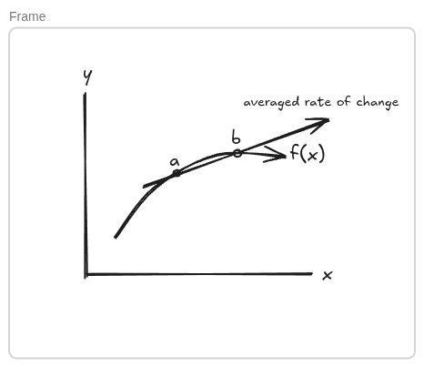
where the line passing through the points $a$ and $b$ can be expressed by a straight line equation. More specifically, algebraically, if $a$ is written as $a=(x_1,y_1)$ and $b$ is written as $b=(x_2,y_2)$ (since they lie on the $x,y$ plane), algebraically, we have that this line is represented by $\frac{y_2-y_1}{x_2-x_1}x+b$ where x is arbitrary and b is the y-intercept. Ok, cool. Well, if we just move $a$ and $b$ a little bit closer, then we would get something more accurate over a small interval, wouldn’t we? Maybe something like:

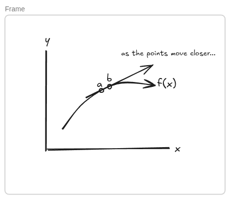
and this will give us a different equation for the straight line passing through $a$ and $b$. From here, we naturally ask, well, can we find the instantaneous rate of change? That is, the rate of change at a single point? And this is where differentiation comes in.

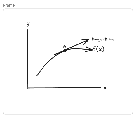
I won’t go into it, but Newton flipped the traditional way of thinking about mathematics (or Gottfried, he doesn’t get enough love) when we ran into the issue of dividing by zero. Namely, pulling up our previous equation: $\frac{y_2-y_1}{x_2-x_1}x+b$ we can see that when we sub in $x_1$ in for $x_2$, we get 0, and that’s a big no no in math. Its, like, the first thing you learn. You just don’t do it. I would go into it about why (the reason is less interesting than you think), but then I would have to explain rings, and that’s outside of the scope of this article.

Anyways, instead of thinking about substituting the raw value in, he thought, well, what if we just looked at the behaviour or pattern as $x_2$ approaches $x_1$? After all, since its assumed that we’re working over the real numbers, we can do that; we can get infinitely closer to $x_1$ without actually touching it. Does it hit a wall? How does it behave?

Using this method, we were able to, through what we know as a mathematical limit, define the derivative; that is, the rate of change, or the tangent line, at a point along a function. Pretty cool! I’m not gonna go into it, but if you’re curious, email me and I’ll yap with you all about it.

Nice.

It took me a while to wrap my head around this, but once I did, I felt pretty great. And now I have to flip it on its head again, because now what we want to look at is the derivative in a multivariate context. Okay, lets try to explain this.

The multivariate derivative

In the classical example, we were working in 2D space; a plotted graph with axis $x$ and $y$. Lets add another dimension, $z$, to spice it up.

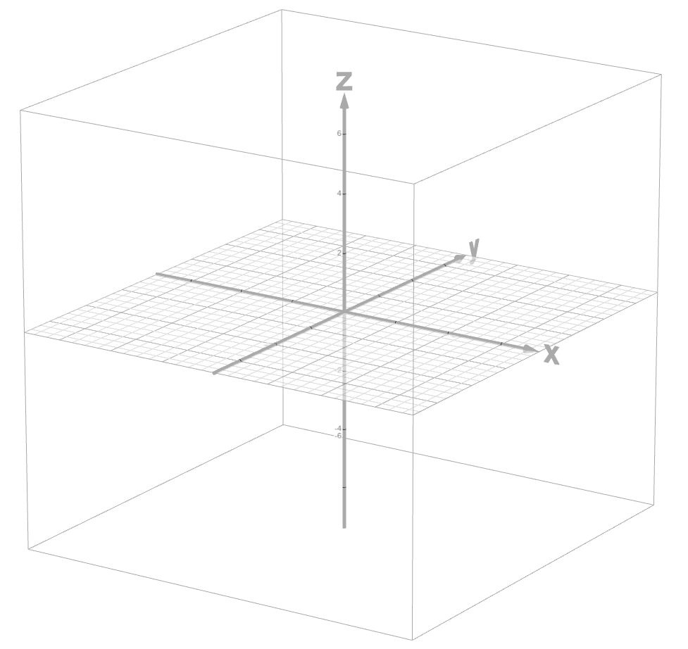
Hey, don’t we just get 3D space?

Yup!

Well, if we can graph objects in 2D space, can’t we also mathematically represent objects in 3D space? Also yes.

Case in point:

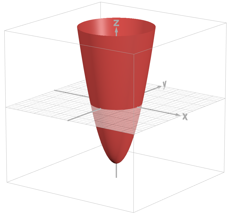
This shape is represented by the equation $z=x^2+y^2-6$ and is formally known as a paraboloid, but that isn’t important. The thing to note here is that we can algebraically express shapes in 3D.

So then, if we wanted to find the derivative at a specific point for this paraboloid, what would that look like?

If we think back to the classical example, we had a straight line that was just touching the point. We can choose a point at which to take the derivative, in this case, I am going to choose (1,1,-4), which looks like this on the paraboloid.

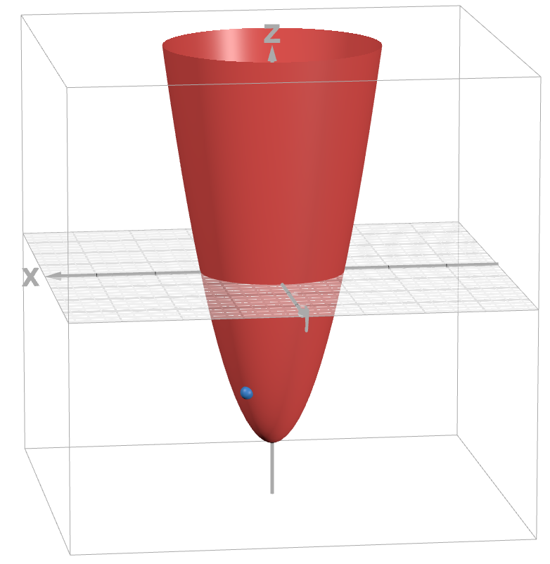
If we apply the same logic in the classical case, then the derivative should be given by the plane just touching the point at the little blue dot, and it will look something like this:

Let’s go into some of the math behind it.

Multivariable derivatives, hard mode (the actual math)

Now that we’ve built our intuition behind the graphical representation of the multivariate derivative, lets see how the actual math hashes out.

It turns out that when we look at the derivative, if we zoom in really closely, we have that for certain points on certain functions, a straight line well approximates that particular portion of the function.

The best example that I can come up with right now is the example of an $n$-sided polygon; we can imagine that, as we add more sides, the polygon gets closer and closer to a circle.

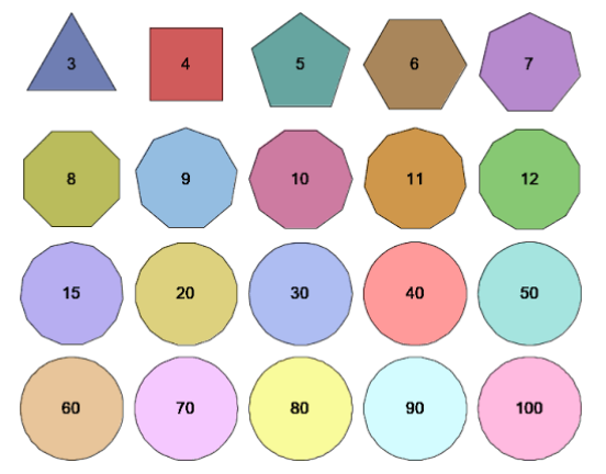
In the $n=100$ case, it looks nearly like a perfect circle; yet, it isn’t a true circle (although the concept of a true circle is something that is thought to only exist in the realm of logic and pure mathematics, not in real life). We can, however, imagine all of those little lines for $n=100$ to be the secant lines of increasingly smaller intervals along a circle. In this scenario, we would be zooming further and further into a specific part of a circle, and we see that as we zoom in closer and closer, the secant line becomes better and better at resembling the actual function at that specific point.

This isn’t true for all functions or shapes; consider a function, like the absolute value function, that is non differentiable at the origin. When we have a sharp corner, we can’t differentiate, because at that point a straight line does not well-approximate the function no matter how far you zoom in.

In general, we can say the following:

• Definition. A function is differentiable at $x=a$ when it is well approximated by a linear function $L(x)$ at $x=a$, i.e. if there exists a straight line $L(x)$ such that it well approximates $f(x)$ at the given point $a$.

Now, we are going to turn our attention away to something slightly different, but will relate back to this concept. Consider a function, we will call it $\vec{f}$, that takes vectors from $R^n$ and sends them to $R^m$. This is an abstract way of putting it, but lets look at an intuitive example; lets go back to our paraboloid.

We have our original paraboloid:

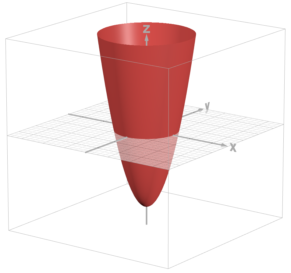
Now, lets tweak with the equation a bit; lets change it to $z=10x^2+5y^2-6$.

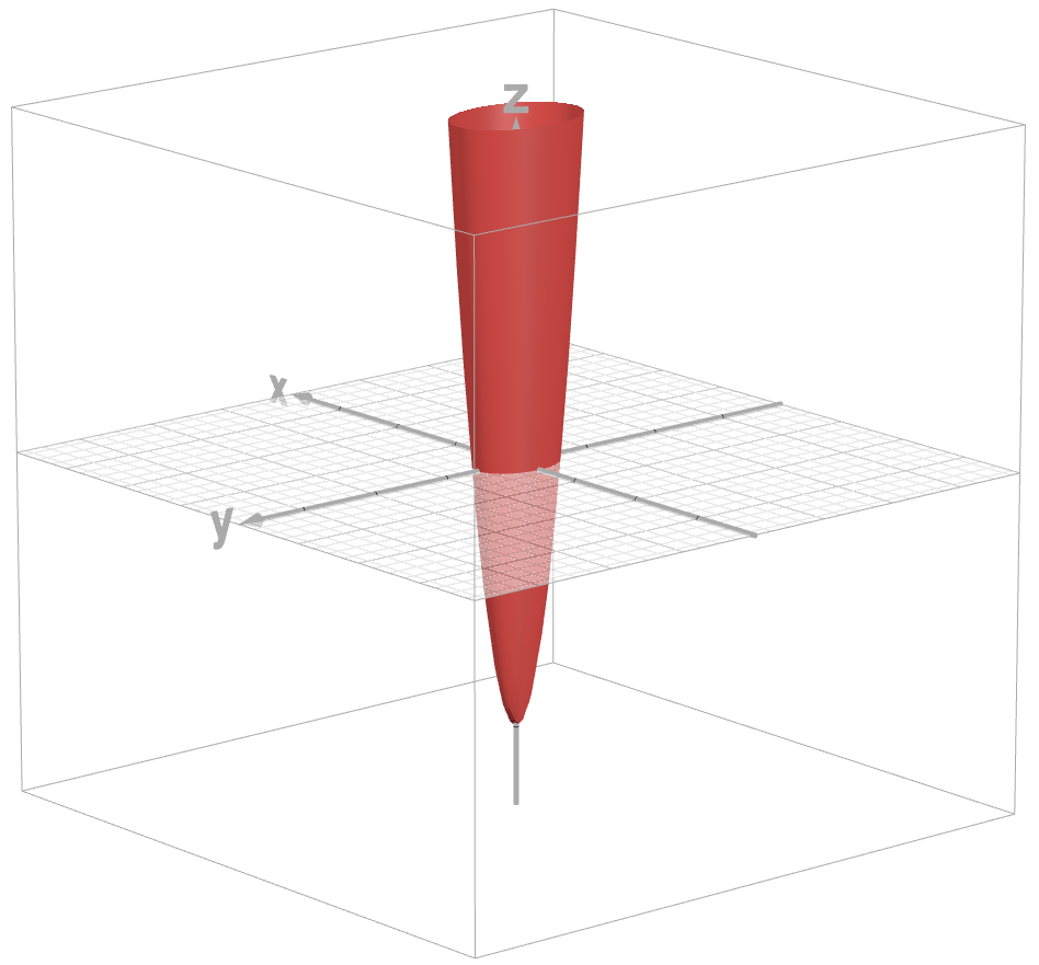
In this case, with respect to what we were talking about earlier, all we did was apply a function on the original paraboloid; that is, the function that shrunk it. We feed in the original shape, it gets crunched through the function, and the skinny paraboloid is the output. In this case, $\vec{f}$ takes vectors in 3D space, modifies them a bit, and then spits out another shape in 3D space. In other words, we have $\vec{f}:R^3\to R^3$. Pretty neat, hey?

But we also could have had the scenario where it gets squished down onto the $x,y$ plane instead, and we might have had something that looked like this:

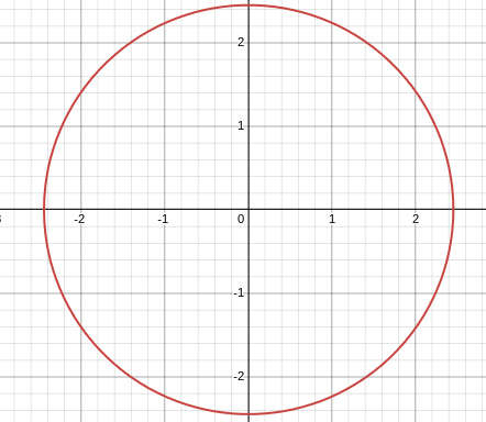
except that the circle would be filled in with all of the points, so just imagine really hard that it is (I couldn’t figure out how to fill it in, and I was spending too much time on it, so I gave up). In this case, we have that $\vec{f}:R^3\to R^2$.

We can also have the other case, where the function adds a dimension, but I really don’t think that I’m smart enough to figure out how to represent that graphically, so I won’t try. My main point here is that $\vec{f}$ is defined as a function that transforms items living in vector spaces, namely, vectors. And when we transform vectors, we can measure the rate at which they change. In other words, we can perform calculus on vectors!

(aka, combining the two maths with the wildest notation/learning curves together and hoping for the best).